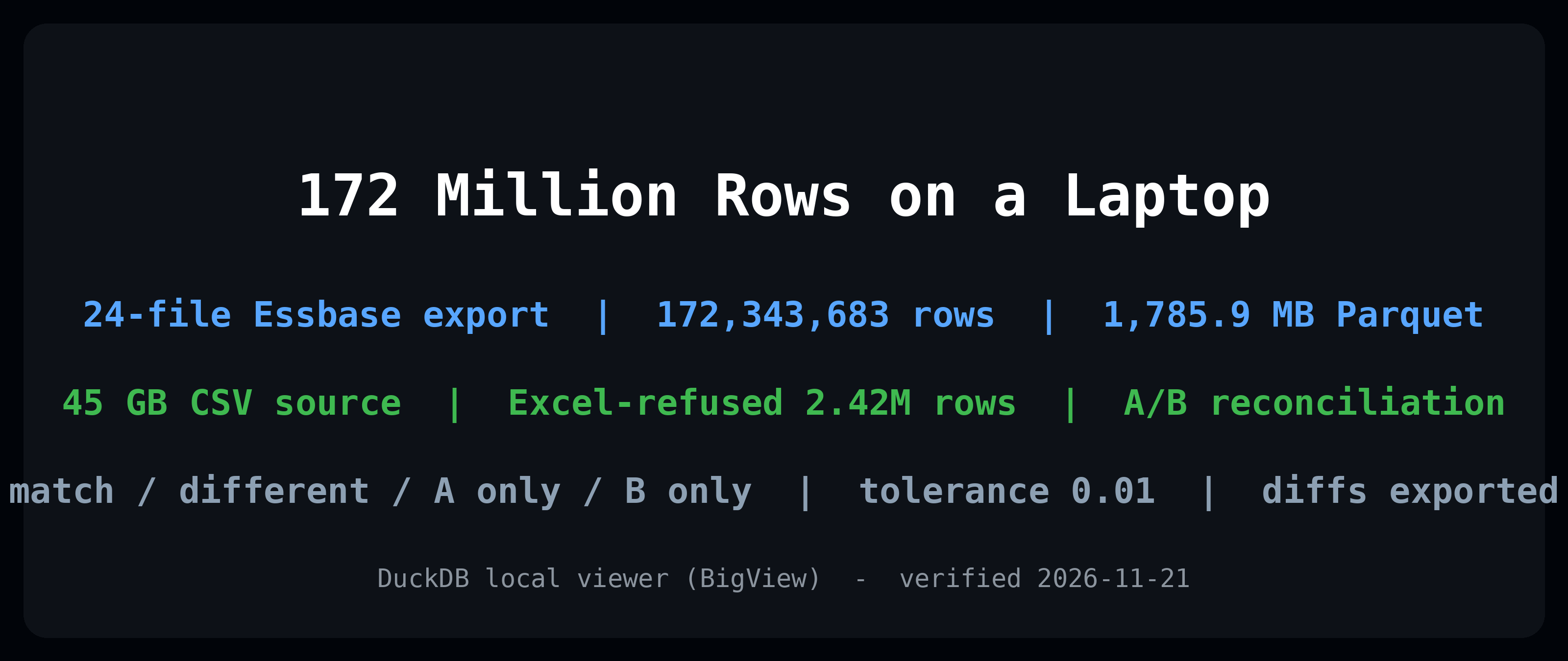
172 Million Rows on a Laptop: Browsing and Reconciling a 45 GB OLAP Export with DuckDB
Environment: a Windows laptop, DuckDB 2.0.1 as the query engine, and a local viewer I built myself (BigView). Every row count and file size in this article comes from a verification run on 2026-11-21 against a real production Essbase export. The one result that comes from synthetic data is labelled synthetic where it appears. You will find no load times or query timings below: I did not run a controlled timing benchmark, so this article reports counts, sizes, and mechanics — the things I actually measured.
The export nobody could open
This started with a smaller file that already broke everything. A colleague exported data from a budgeting system (Essbase / Hyperion Planning) as CSV: 2,422,632 rows in JLBAPP_DATA.csv. Excel’s hard limit is 1,048,576 rows per worksheet, so Excel did not open it slowly or partially — it refused. The generic “large CSV viewer” tools I tried either loaded the whole file into memory and died, or were database tools that expected me to write SQL before I could look at a single row.
Then came the real problem: a full export of the same system, roughly 45 GB of CSV. Not a file you open — a file you deal with.
The frustrating part is what the job actually was. I did not need a data platform. I needed to look at the export before trusting it: scroll it, filter one column, check whether a specific member’s values were there, and later — the recurring task in OLAP consulting work — compare two versions of an export and answer one question: what changed? When a calculation rule is modified and the cube is re-exported, somebody has to prove the new export differs from the old one only where it should. That proof is usually attempted in a spreadsheet, on data the spreadsheet cannot hold.
So I built the tool I needed: a local viewer with DuckDB as the engine. It grew into a product I call BigView. This article is the verification story — what the tool was tested against, how its reconciliation mode works down to the SQL, and the boundaries I am not going to pretend away.
The design rule: the browser never holds the data
The architecture follows one rule: the file lives in DuckDB, and the screen only ever holds the few hundred rows you are looking at.
On open, the file is registered with DuckDB. After that, every interaction is a small SQL query against the file in place:
- Scrolling fetches a window of rows around the visible position (
LIMIT/OFFSET); the grid renders only that window, no matter how many millions of rows sit behind it. - Sorting and filtering are pushed down into SQL. The browser never filters locally — it cannot, it does not have the data.
- Find is a
row_number()window query over the current view: it returns the positions of the hits, so the grid can jump to each one. (Window functions doing unglamorous plumbing work is a recurring theme; our complete guide to DuckDB window functions covers the machinery.)
This works because of how DuckDB reads files: columnar scanning and predicate pushdown mean a query touches the columns and row groups it needs instead of hauling the whole file into memory (the pushdown behaviour DuckDB’s own Parquet documentation describes) — the same principles we benchmarked in DuckDB vs Pandas for large files. The viewer is a thin local web app on top of that engine: a Python standard-library HTTP server, one HTML file, and DuckDB. It binds to 127.0.0.1. The exports it opens are financial data, so the tool makes no network calls and the data never leaves the machine. That is not a feature bullet; for this class of file it is the entry requirement.
The real test: 172,343,683 rows
A viewer that opens a 2.4-million-row CSV has proven something modest. The 45 GB export is the test that matters, so that is what I verified it against.
The export was converted to Parquet — one folder, 24 files, one per cube extract. The folder is the natural unit here: an OLAP export is never one file, and any tool that insists on a single file at a time forces you to verify an export in 24 disconnected pieces. The verified figures:
| Item | Rows | Size |
|---|---|---|
| Plan1_3.parquet | 7,285,224 | — |
| Plan1_4.parquet | 7,693,628 | — |
| Plan1_13.parquet | 6,244,879 | — |
| All 24 Parquet files | 172,343,683 | 1,785.9 MB |
| Source export (CSV) | — | ≈ 45 GB |
Each of the three named files opens and browses directly on its own — six to seven million rows is already six times past Excel’s limit — and the folder as a whole opens as one logical table of 172,343,683 rows. That last part is not a viewer trick; it is the entry point to the feature this article is really about.
Two honest qualifications. First, these are row counts and byte counts, not speeds: the verification established that the full export opens, browses, and reconciles on a laptop, not how it would score in a benchmark harness. Second, Parquet is doing heavy lifting in this story — 1,785.9 MB of columnar files is a different proposition from 45 GB of CSV text, and converting the export is a step I control in my own workflow. If your export pipeline only produces CSV, the viewer still opens the files; the folder-level reconciliation described below is the part that is built on Parquet.
Reconciliation mode: two folders, one verdict
Browsing answers “what is in this export?” The question that recurs in practice is comparative: “I have last week’s export and this week’s export — did the rule change I shipped move anything it should not have?” In V8 the viewer grew a reconciliation mode for exactly that. You point it at two folders — side A and side B — and it treats each folder as one logical table.
Step 1 — A folder becomes a table
Each side is a DuckDB view over every Parquet file in the folder:
CREATE VIEW side_a AS
SELECT * FROM read_parquet('export_a/*.parquet', union_by_name = true);

CREATE VIEW side_b AS
SELECT * FROM read_parquet('export_b/*.parquet', union_by_name = true);
union_by_name = true is the load-bearing parameter. Files in a real export folder do not all share an identical column set — an extract added mid-year, a column one cube has and another does not. A plain union fails on the first mismatch; union_by_name aligns columns by name and fills the gaps with NULL, which is the behaviour you want when the alternative is the comparison not running at all. DuckDB documents this schema-unification behaviour in its guide to reading multiple files. The 24-file, 172-million-row folder above is one of these views.
Step 2 — Aggregate to a common grain, then full outer join
The comparison aggregates both sides to the same key grain — the member intersection you are checking — and joins them with a FULL OUTER JOIN, because the interesting rows are precisely the ones that exist on only one side:
WITH a AS (SELECT <key columns>, sum(value) AS va FROM side_a GROUP BY ALL),
     b AS (SELECT <key columns>, sum(value) AS vb FROM side_b GROUP BY ALL)
SELECT
    coalesce(a.<key>, b.<key>) AS key,
    CASE
        WHEN a.va IS NULL THEN 'B only'
        WHEN b.vb IS NULL THEN 'A only'
        WHEN abs(a.va - b.vb) <= 0.01 THEN 'match'
        ELSE 'different'
    END AS status,
    a.va, b.vb, b.vb - a.va AS diff
FROM a FULL OUTER JOIN b USING (<key columns>);
Every compared intersection lands in exactly one of four classes: match, different, A only, or B only. The report is the class counts, the total of side A, the total of side B, and the net difference — so a comparison that “mostly matches” still has to show its arithmetic. The boundary between match and different is an absolute tolerance of 0.01: at currency scale, sub-cent representation noise should not page anyone, and anything above it is a real difference that gets listed. The differing rows export to CSV, because a verdict without the row list is just an opinion — the follow-up work happens on those exact intersections.
This is the same discipline as the zero-diff reconciliation method we use for offline replicas: a difference is only useful if it localizes to precise members. The tolerance differs (0.01 here, exactly zero there) because the questions differ — that method proves a replica is faithful; this mode triages two exports so a human can start from the short list of what actually moved.
The grain decision, and why the report shows more than the net
Two design choices in that SQL are worth spelling out, because they decide whether the verdict means anything.
First, both sides are aggregated before the join, not compared row by row. A level-0 export carries one row per full member intersection; comparing at that grain produces a diff list as long as the export itself. Aggregating both sides to the grain you actually intend to sign off — say, account by entity by month — makes the four classes readable: a “different” row is a place a human can go and look. You can always re-run at a finer grain on the segment that failed; you cannot un-drown a report that started at maximum detail.
Second, the net difference is the least informative number in the report, and it is shown alongside the class counts and both side totals precisely so it cannot be read alone. Two exports can net to zero while hundreds of intersections moved in offsetting directions — a reallocation between entities, for instance, is invisible in the net and obvious in the “different” count and the exported row list. Conversely, a large net with zero “different” rows and a block of “A only” rows tells a different story: something was added or dropped wholesale, not revalued. The classes are the diagnosis; the net is just the checksum.
Step 3 — What the functional test showed
Before pointing the mode at real exports, I ran it against a small synthetic pair of folders with planted differences — keys designed to hit every class. The classification came back:
| Class | Count |
|---|---|
| Match | 45 |
| Different | 2 |
| A only | 1 |
| B only | 1 |
That is a synthetic functional test — it proves the classification logic sorts planted cases into the right buckets, nothing more. It is deliberately not dressed up as a business result. The real-data verification is the 172-million-row folder above: the mode’s views and comparisons run against the same production export the viewer was validated on, at full scale, on the laptop.
Where it stops
A hands-on report that only lists capabilities is an advertisement, so here are the boundaries, plainly:
- Read-only, no write-back. The viewer and the reconciliation mode inspect exports. Data entry and official calculation stay in the system of record; nothing here writes back to a cube, and a reconciliation report is evidence for a decision, not the decision applied.
- One machine, one user. This is a local tool. There is no shared server, no concurrent multi-user access, no collaboration. If your team needs ten people diffing exports simultaneously, you need a platform, not a viewer.
- No security semantics travel with an export. The source system’s permissions and filters do not exist in a folder of Parquet files. Whoever holds the folder holds the data — handle exports accordingly.
- Local resources are the ceiling. The folder has to fit on your disk, and very wide comparisons are bounded by your machine’s memory and DuckDB’s spill behaviour. The knobs that govern that —
memory_limit, threads, temporary directory — are the same ones covered in our DuckDB performance tuning guide; the viewer does not repeal them. - It is not an ETL tool and not a benchmark. It does not transform, schedule, or pipeline anything. It opens, shows, and compares.
Who this is for
The pattern that produced this tool is common in OLAP and finance work: you do not get access to the system, you get the export. EPM consultants verifying that a rule change moved only the intended intersections; finance engineers handed a migration extract and asked to sign off on it; anyone whose interface to a large system is a folder of files too big for the spreadsheet on their desk. For that work, the useful unit is not a database — it is a tool that opens the whole export, lets you look at any of it, and reduces “what changed?” to a four-class verdict with a row list attached.
The viewer is BigView. The numbers above are the whole claim: a 2,422,632-row CSV that Excel refused, a 24-file production export totalling 172,343,683 rows and 1,785.9 MB browsed as a single table on a laptop, and a reconciliation mode that classifies every compared intersection as match, different, A only, or B only — with the differences exported, not asserted. Everything else a tool in this category promises, you should ask it to show you in the same currency: rows, files, and the diff list.
Further reading
- Zero-Diff Reconciliation: proving a DuckDB copy of enterprise data is correct — the stricter method this mode’s triage complements
- DuckDB vs Pandas for large log files — columnar scanning and predicate pushdown, benchmarked
- DuckDB performance tuning: 5 tips — the memory and parallelism knobs that bound local work
- DuckDB window functions: the complete guide — including the
row_number()machinery behind the viewer’s find