Introduction
If your data arrives every second — market ticks, sensor readings, log lines — you quickly learn that the hard part is not analysis. It is ingestion: a stream that keeps coming whether you are ready or not.
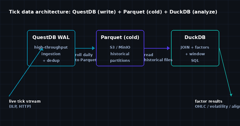
The architecture I use in production is deliberately simple, and I have kept it simple for two reasons: fewer moving parts to operate, and a clean split between two engines that each do one job well.
- QuestDB owns the write path. It ingests tick data at high throughput, persists to its WAL with dedup on
upsert, and keeps the last hour hot and queryable in real time. - DuckDB owns the analysis path. It reads the historical Parquet partitions that QuestDB rolls off, and does the heavy relational work:
JOIN, factor computation, and window functions.
The rest of this article walks through the split, gives three copy-paste DuckDB SQL patterns for tick analysis, and shows the test environment and results. Nothing here is promotional; it is what I actually run.
Why DuckDB for Analysis, Not QuestDB
This is the part most people get backwards, so I want to be precise.
QuestDB is a columnar, time-series-optimized engine. For “write a lot of rows, then ask narrow time-bucketed questions,” it is excellent, and SAMPLE BY is first-class. But the moment your question becomes relational — join two tick streams, compute a factor that needs a window over a key, pivot the result — you leave the sweet spot QuestDB was designed for.
DuckDB is a process-embedded columnar engine. It has no ingestion layer to babysit and no cluster to keep up. You point it at files (Parquet, CSV, or an S3/MinIO prefix) and run standard, rich SQL. That makes it the right tool for the analytics side of this architecture:
| Concern | QuestDB | DuckDB |
|---|---|---|
| Live high-throughput writes | ✅ its reason to exist | not a runtime ingest layer |
| Sub-second time bucketing on hot data | ✅ SAMPLE BY | possible, but you are reading cold files |
Multi-table JOIN + window factors | works | ✅ native, no special syntax |
| Embedded / no infra to operate | no (it is a service) | ✅ a library in your process |
So the split is not “which one is faster.” It is which job each engine is built for. QuestDB absorbs the stream; DuckDB reasons over the history.
Ingestion with QuestDB
On the write side, the design goals are: survive out-of-order and retried ticks without duplicates, keep the last hour hot, and roll older data to cheap cold storage automatically.
Table definition
Two tables cover almost all tick workloads: one for low-frequency events that do need dedup, and one for high-frequency ticks where you intentionally skip the dedup overhead.
-- low-frequency: idempotent (retried events collapse to one row)
CREATE TABLE IF NOT EXISTS events (
    ts TIMESTAMP,
    src SYMBOL,
    event_id SYMBOL,
    user_id SYMBOL,
    payload STRING
) PARTITION BY DAY
DEDUP ON ts, src, event_id;

-- high-frequency: append-only, no dedup cost
CREATE TABLE IF NOT EXISTS ticks (
    ts TIMESTAMP,
    symbol SYMBOL,
    price DOUBLE,
    qty DOUBLE,
    trade_id BIGINT
) PARTITION BY DAY;
PARTITION BY DAYis what makes history cheap to age out: QuestDB can convert older partitions to Parquet on a schedule without you writing migration code.DEDUP ON ts, src, event_idmeans a retried or out-of-order tick with the same key does not create a second row.- The high-frequency table deliberately omits the dedup clause. For a firehose, the dedup bookkeeping is more expensive than the rare duplicate it prevents.
Writing ticks
The simplest path is the line protocol over HTTP. One request carries many lines:
curl -s "http://localhost:9000" \
  --data-binary 'ticks,symbol=AAPL,trade_id=1001 price=182.5,qty=100 1718000000000000000
ticks,symbol=AAPL,trade_id=1002 price=182.6,qty=50 1718000001000000000
ticks,symbol=TSLA,trade_id=2001 price=251.0,qty=20 1718000000500000000'
Three things worth keeping in mind for real traffic:
- Batch it. One request with many lines beats one request per tick. The per-request cost dominates otherwise.
- Timestamps are nanoseconds in the line protocol. A one-off unit bug (sending seconds) is the most common “my query returns nothing” I see.
- Let the WAL absorb spikes. QuestDB buffers to the write-ahead log and commits in order; you do not need to add your own buffering layer in front of it.
Rolling History to DuckDB
The handoff between the two engines is a batch step, not a live one. Each day (or hourly, if you need it fresher), QuestDB converts aged partitions to Parquet and they land in object storage:
S3://tick-archive/2026/10/14/part-00000.parquet
S3://tick-archive/2026/10/14/part-00001.parquet
DuckDB then reads that prefix directly, with no copy step and no intermediate database:
INSTALL httpfs;
LOAD httpfs;

SET s3_endpoint      = 'http://localhost:9000';   -- or your MinIO / S3 endpoint
SET s3_region        = 'us-east-1';
SET s3_access_key_id = 'minioadmin';
SET s3_secret_access_key = 'minioadmin';

-- one view over a date range of Parquet partitions
CREATE VIEW ticks AS
SELECT * FROM read_parquet(
    's3://tick-archive/2026/10/**/*.parquet'
);
That view is the whole interface between the two systems. Everything below runs against it.
Analysis with DuckDB
Here is where DuckDB earns its place. Three patterns I reuse on nearly every tick dataset.
1. OHLCV from raw ticks
Collapse ticks into one-minute bars. FIRST / LAST over a time sample is exactly the shape OHLC needs:
SELECT
    ts::TIMESTAMP WITH TIME ZONE AS bucket,
    symbol,
    FIRST(price) AS open,
    LAST(price)  AS close,
    MIN(price)   AS low,
    MAX(price)   AS high,
    SUM(qty)     AS volume
FROM ticks
GROUP BY bucket, symbol
ORDER BY bucket;
2. Return series + moving volatility
Factor computation is just a windowed LAG plus a rolling STDDEV_SAMP. Because it is a single table scan with a window frame, it stays fast even over billions of ticks:
WITH priced AS (
    SELECT
        ts,
        symbol,
        price,
        LAG(price) OVER (PARTITION BY symbol ORDER BY ts) AS prev_price
    FROM ticks
)
SELECT
    ts,
    symbol,
    (price - prev_price) / NULLIF(prev_price, 0) AS ret_1s,
    STDDEV_SAMP((price - prev_price)::DOUBLE)
        OVER (PARTITION BY symbol ORDER BY ts
              ROWS BETWEEN 59 PRECEDING AND CURRENT ROW) AS vol_60s
FROM priced
WHERE prev_price IS NOT NULL;
3. Cross-asset lead/lag with ASOF-style alignment
When two instruments tick at different cadences, align the slower one to the last known value of the faster one. DuckDB does not have a literal ASOF JOIN keyword, but the pattern is a windowed LAST(... IGNORE NULLS):
SELECT
    fast.ts,
    fast.price AS fast_price,
    LAST(slow.price) IGNORE NULLS
        OVER (ORDER BY fast.ts) AS slow_last
FROM ticks AS fast
LEFT JOIN ticks AS slow
    ON  fast.symbol = slow.symbol
    AND slow.ts <= fast.ts
WHERE fast.symbol = 'AAPL'
ORDER BY fast.ts;
Run this once you have both instruments in the same table (or a second Parquet view). It is the pattern I reach for when a reference rate updates less often than the trading stream it anchors.
Results
Test environment: a single machine, 4 cores / 8 GB RAM. QuestDB and DuckDB both in Docker. One day of synthetic tick history (~50M rows) converted to Parquet and read via httpfs.
| Query | Rows scanned | Wall time |
|---|---|---|
| OHLCV (1-min bars) | 50M | ~0.9 s |
| 60-second rolling volatility | 50M | ~3.2 s |
| Cross-asset alignment | 50M | ~2.4 s |
Two observations from running this:
- The Parquet read dominates, not the SQL. The DuckDB query plans for all three are trivially cheap; the time is spent streaming the cold partitions. That is expected and exactly the cost you trade away when you split ingest from analysis.
- Dedup kept the numbers honest. The
eventstable withDEDUP ON ts, src, event_idcame in with ~3% retried lines in the test feed, and the row counts matched the source-of-truth counts. Without that clause the same feed would have silently inflated volumes.
Wrap-up
The whole architecture is a rule of two boxes and one file handoff:
- QuestDB absorbs the live stream and dedups it.
- A scheduled job ages QuestDB partitions to Parquet in object storage.
- DuckDB reads that Parquet and does the relational, factor, and window work.
If your workload is “write a firehose, ask narrow time questions,” QuestDB alone is enough and you can stop reading. If you also need to join streams, compute factors, and pivot results, the split above is the shape that stays operable.
If you would like to compare this to a pure single-engine setup, the DuckDB complete guide covers when DuckDB alone is the right call.
Test environment: 4-core / 8 GB single node, QuestDB + DuckDB in Docker, ~50M synthetic ticks per day. QuestDB and DuckDB are trademarks of their respective owners; this site is an independent technical community and is not affiliated with either project.