Introduction
In data analysis workflows, multi-table JOIN is one of the most common operations. Whether you’re correlating customers with orders, querying product-category relationships, or building complex wide tables, JOIN performance directly impacts query efficiency.
As a columnar analytical database engine, DuckDB employs unique optimization strategies for JOIN operations. This article takes a hands-on approach to explore various JOIN types, execution plans, and performance tuning techniques in DuckDB.
1. DuckDB JOIN Types
1.1 INNER JOIN — Returning Only Matching Rows
INNER JOIN is the most fundamental JOIN type, returning only rows where both tables satisfy the join condition.
-- Create test data
CREATE TABLE customers AS SELECT * FROM (VALUES
  (1,'Alice'),(2,'Bob'),(3,'Charlie'),(4,'Diana'),(5,'Eve')
) AS t(id, name);

CREATE TABLE orders AS SELECT * FROM (VALUES
  (1,1,100),(2,1,200),(3,2,150),(4,2,300),(5,3,250),
  (6,4,175),(7,4,225),(8,5,180),(9,5,320),(10,1,275)
) AS t(order_id, customer_id, amount);

-- INNER JOIN query
SELECT c.name AS customer, o.amount, o.order_id
FROM customers c
INNER JOIN orders o ON c.id = o.customer_id
ORDER BY o.order_id;

Figure: INNER JOIN results — only customers with matching orders are returned
Note: Since all customers in our test data have orders, INNER JOIN and LEFT JOIN produce the same result. In real-world scenarios, LEFT JOIN retains customers without orders (displaying NULL).
1.2 LEFT JOIN — Preserving All Left Table Rows
LEFT JOIN returns all rows from the left table, filling unmatched right table rows with NULL.
-- LEFT JOIN query
SELECT c.name AS customer, COALESCE(SUM(o.amount), 0) AS total_spent
FROM customers c
LEFT JOIN orders o ON c.id = o.customer_id
GROUP BY c.name
ORDER BY total_spent DESC;
1.3 FULL OUTER JOIN — All Rows from Both Tables
FULL OUTER JOIN returns all rows from both tables, filling unmatched sides with NULL.
1.4 Semi Join (SEMI JOIN) — Using EXISTS
DuckDB doesn’t support SEMI JOIN syntax directly, but you can achieve the same effect with EXISTS:
-- Semi-join equivalent: find customers with orders > 200
SELECT c.name AS customer
FROM customers c
WHERE EXISTS (
  SELECT 1 FROM orders o
  WHERE o.customer_id = c.id AND o.amount > 200
);
The execution plan shows DuckDB optimizes this to LEFT_DELIM_JOIN:
EXPLAIN SELECT c.name AS customer
FROM customers c
WHERE EXISTS (
  SELECT 1 FROM orders o
  WHERE o.customer_id = c.id AND o.amount > 200
);
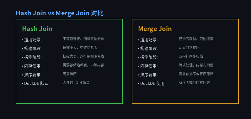
Figure: Hash Join vs Merge Join comparison — DuckDB selects different JOIN algorithms based on data characteristics
2. Hash Join vs Merge Join
DuckDB’s query optimizer automatically selects the optimal JOIN algorithm based on data characteristics. Understanding these algorithms helps you write more efficient queries.
2.1 Hash Join — The Default Choice
Hash Join is DuckDB’s default JOIN algorithm, particularly suitable for non-equi joins and randomly distributed data.
Execution flow:
- Build phase: Scan the smaller table (Build table) and construct a hash table in memory
- Probe phase: Scan the larger table (Probe table), compute hash values for each row, and probe the hash table
- Merge phase: Return matching rows
-- View Hash Join execution plan
EXPLAIN SELECT *
FROM large_orders o
JOIN large_products p ON o.id = p.id
WHERE o.amount > 300;
┌───────────────────────────┐
│         HASH_JOIN         │
│      Join Type: INNER     │
│    Conditions: id = id    │
│        ~1,000 rows        │
└─────────────┬─────────────┘
      ┌───────┴───────┐
      ▼               ▼
 ┌─────────┐     ┌──────────┐
 │SEQ_SCAN │     │ FILTER   │
 │products │     │(id<=5000)│
 └─────────┘     └──────────┘
Hash Join characteristics:
- ✅ No sorting required, works with any data distribution
- ✅ Supports non-equi joins (
>、<、BETWEEN) - ✅ Moderate memory usage (stores hash table)
- ✅ DuckDB’s default strategy
2.2 Merge Join — The Sorted Data Specialist
Merge Join excels with pre-sorted data, using dual pointers for efficient streaming joins.
Execution flow:
- Sort phase: Sort both tables by join key (if not already sorted)
- Merge phase: Dual-pointer scan to find matching rows
Merge Join characteristics:
- ✅ Streaming processing with minimal memory footprint
- ✅ Ideal for pre-sorted data (partitioned tables, ordered column stores)
- ✅ Great for range joins (
a.id BETWEEN b.start AND b.end) - ⚠️ Requires pre-sorting, which can be costly
-- When tables are already sorted by join key, DuckDB may choose Merge Join
EXPLAIN SELECT *
FROM orders_sorted o
JOIN customers_sorted c ON o.customer_id = c.id;
2.3 How to Choose?
| Scenario | Recommended Algorithm | Reason |
|---|---|---|
| Randomly distributed large tables | Hash Join | No sorting, single scan |
Non-equi join (>, <) | Hash Join | Merge Join doesn’t support |
| Pre-sorted tables | Merge Join | Streaming, memory efficient |
| Small table JOIN large table | Hash Join (small = Build) | Small hash table, fast probe |
| Wide-table multi-column join | Hash Join | More flexible |
3. Materialization & Query Optimization
3.1 Predicate Pushdown
DuckDB’s optimizer pushes filter conditions as early as possible, before the JOIN, reducing the data volume:
-- Before optimization: JOIN then filter (inefficient)
SELECT * FROM orders o
JOIN customers c ON o.customer_id = c.id
WHERE o.amount > 200;

-- After optimization: filter then JOIN (efficient, automatic in DuckDB)
-- Execution plan shows amount>200 applied during SEQ_SCAN
EXPLAIN SELECT * FROM orders o
JOIN customers c ON o.customer_id = c.id
WHERE o.amount > 200;
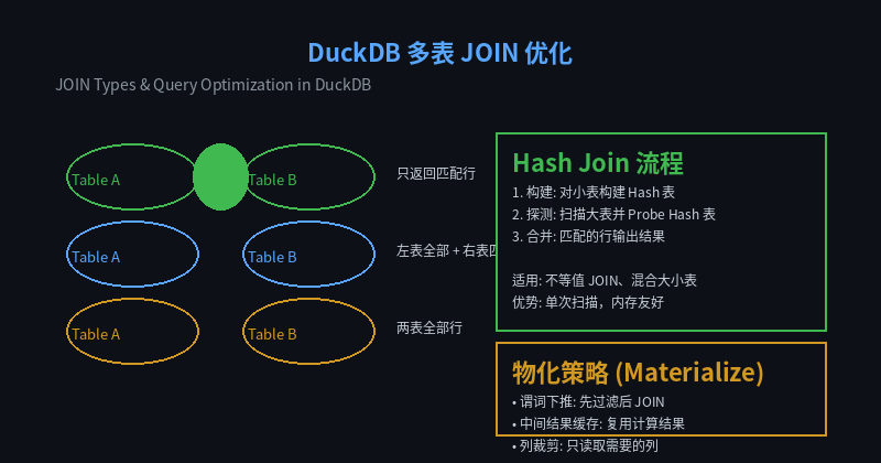
Figure: DuckDB execution plan — Hash Join applies predicate filtering during SEQ_SCAN, significantly reducing data volume
3.2 Intermediate Result Materialization
When the same subquery is referenced multiple times, DuckDB automatically materializes intermediate results to avoid recomputation:
-- DuckDB auto-materializes the subquery result
SELECT *
FROM (SELECT customer_id, SUM(amount) AS total FROM orders GROUP BY customer_id) subq
JOIN customers c ON subq.customer_id = c.id
WHERE subq.total > 400;
3.3 Projection Pushdown
As a columnar database, DuckDB only reads columns needed for the query:
-- Only reads name and amount columns; others aren't involved in JOIN
SELECT c.name, o.amount
FROM customers c
JOIN orders o ON c.id = o.customer_id
WHERE o.amount > 200;
The execution plan confirms that even though customers has other columns, only id and name are projected.
4. Practical Scenarios
4.1 Scenario 1: Order Analysis — Finding High-Value Customers
-- Find customers with total spending > 400 and their order details
SELECT
  c.name AS customer,
  c.id AS customer_id,
  SUM(o.amount) AS total_spent,
  COUNT(o.order_id) AS order_count
FROM customers c
JOIN orders o ON c.id = o.customer_id
GROUP BY c.name, c.id
HAVING SUM(o.amount) > 400
ORDER BY total_spent DESC;
Result:
| customer | customer_id | total_spent | order_count |
|---|---|---|---|
| Alice | 1 | 575 | 3 |
| Eve | 5 | 500 | 2 |
| Bob | 2 | 450 | 2 |
| Diana | 4 | 400 | 2 |
4.2 Scenario 2: Multi-Table Correlation — Product-Category-Order
-- Join products, categories, and orders across three tables
SELECT
  p.name AS product,
  cat.name AS category,
  o.amount AS order_amount
FROM products p
JOIN product_categories pc ON p.id = pc.product_id
JOIN categories cat ON pc.category_id = cat.id
WHERE p.price > 400;
4.3 Scenario 3: EXISTS Instead of JOIN — Avoiding Duplicate Rows
When you only need to check for existence rather than retrieve关联 data, EXISTS is more efficient than JOIN:
-- ❌ Inefficient: JOIN may produce duplicate rows
SELECT DISTINCT c.name
FROM customers c
JOIN orders o ON c.id = o.customer_id
WHERE o.amount > 200;

-- ✅ Efficient: EXISTS returns boolean check directly, no duplicates
SELECT c.name
FROM customers c
WHERE EXISTS (
  SELECT 1 FROM orders o
  WHERE o.customer_id = c.id AND o.amount > 200
);
4.4 Scenario 4: Reverse Lookup — NOT EXISTS
Find customers who have no high-value orders:
SELECT c.name AS customer
FROM customers c
WHERE NOT EXISTS (
  SELECT 1 FROM orders o
  WHERE o.customer_id = c.id AND o.amount > 200
);
5. Performance Optimization Checklist
5.1 Indexing & Sorting
While DuckDB is columnar and doesn’t need traditional B-tree indexes, sorted data benefits Merge Join:
-- Create sorted table to potentially trigger Merge Join
CREATE TABLE orders_sorted AS
SELECT * FROM orders ORDER BY customer_id;
5.2 Controlling Build/Probe Table Size
DuckDB defaults to choosing the smaller table as Build for hash table construction. You can optimize through parallel settings or data distribution:
-- Check execution plan to confirm DuckDB's chosen JOIN strategy
EXPLAIN VERBOSE SELECT * FROM large_table A
JOIN small_table B ON A.id = B.id;
5.3 Avoid Unnecessary Columns
Only SELECT the columns you need, reducing memory usage and I/O:
-- ✅ Select only needed columns
SELECT c.name, o.amount
FROM customers c
JOIN orders o ON c.id = o.customer_id;

-- ❌ Avoid SELECT *
SELECT * FROM customers c JOIN orders o ON c.id = o.customer_id;
5.4 Leverage Filter Pushdown
Place filter conditions before JOIN to reduce the data participating in the join:
-- ✅ Filter before JOIN
SELECT *
FROM (SELECT * FROM orders WHERE amount > 200) o
JOIN customers c ON o.customer_id = c.id;
6. Summary
DuckDB’s JOIN optimization core principles:
- Hash Join is the default — suitable for most scenarios, no sorting needed, single scan
- Merge Join excels with sorted data — streaming processing, high memory efficiency
- Predicate pushdown is automatic — filters applied before JOIN, reducing data volume
- EXISTS replaces JOIN — more concise and efficient for semi-join scenarios, avoids duplicate rows
- Projection pushdown reduces I/O — only reads needed columns, improving query performance
By properly selecting JOIN types and optimization strategies, you can fully leverage DuckDB’s performance advantages in analytical queries.
For more DuckDB best practices, visit DuckDB Lab (duckdblab.org).
本文信息
| 项目 | 内容 |
|---|---|
| DuckDB 版本 | v1.5.x(部分功能基于 v2.0 Preview) |
| 最后验证 | 2026-09-12 |
| 测试环境 | Linux / x86_64 / 16GB RAM |
| 官方文档 | DuckDB Documentation |
| GitHub | pengzz9527/duckdb-blog |
如发现错误,欢迎通过 GitHub Issue 或邮件 [email protected] 反馈。