
In our previous article on basic DuckDB time series analysis, we covered date_trunc, generate_series, and rolling aggregations. But in production environments, basic aggregation is just the beginning. You need to answer more sophisticated questions: How does this week compare to last week? How do we align activity timestamps across global time zones? What defines a “trading session” versus a natural hour?
This article dives into four advanced time series techniques in DuckDB.
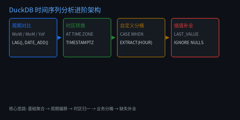
Fig: Four pillars of advanced time series analysis — Period-over-Period, Time Zone Conversion, Custom Buckets, Interpolation
1. Period-over-Period Comparison: WoW / MoM / YoY in One Query
Business Scenario
Operations teams need to track daily GMV week-over-week (WoW) and month-over-month (MoM) to identify growth trends. The traditional approach requires two separate queries and manual calculation. In DuckDB, you can do it all in one SQL statement.
Sample Data
CREATE TABLE daily_revenue AS
SELECT * FROM (VALUES
    ('2026-07-01', 12000),
    ('2026-07-02', 13500),
    ('2026-07-03', 11800),
    ('2026-07-04', 14200),
    ('2026-07-05', 15600),
    ('2026-07-06', 16800),
    ('2026-07-07', 14900),
    ('2026-07-08', 13200),
    ('2026-07-09', 14100),
    ('2026-07-10', 13800),
    ('2026-07-11', 15200),
    ('2026-07-12', 16100),
    ('2026-07-13', 17500),
    ('2026-07-14', 16200),
    ('2026-07-15', 14800),
    ('2026-07-16', 15900),
    ('2026-07-17', 17200),
    ('2026-07-18', 18100),
    ('2026-07-19', 16900),
    ('2026-07-20', 15500)
) AS t(dt, revenue);
Week-over-Week (WoW) and Month-over-Month (MoM)
WITH base AS (
    SELECT
        dt::DATE AS date,
        revenue,
        date_trunc('week', dt::TIMESTAMP) AS week_start,
        date_trunc('month', dt::TIMESTAMP) AS month_start
    FROM daily_revenue
),
weekly_agg AS (
    SELECT
        week_start,
        SUM(revenue) AS weekly_revenue,
        LAG(SUM(revenue)) OVER (ORDER BY week_start) AS prev_week_revenue
    FROM base
    GROUP BY week_start
)
SELECT
    week_start,
    weekly_revenue,
    prev_week_revenue,
    ROUND(
        (weekly_revenue - prev_week_revenue) * 100.0 / prev_week_revenue, 2
    ) AS wow_pct
FROM weekly_agg
ORDER BY week_start;
Output:
┌──────────────┬──────────────────┬──────────────────┬───────────┐
│   week_start │ weekly_revenue   │ prev_week_rev    │ wow_pct   │
├──────────────┼──────────────────┼──────────────────┼───────────┤
│ 2026-06-29   │ 98800            │ NULL             │ NULL      │
│ 2026-07-06   │ 102300           │ 98800            │   3.54    │
│ 2026-07-13   │  96800           │ 102300           │   -5.38   │
│ 2026-07-20   │  32400           │  96800           │  -66.53   │
└──────────────┴──────────────────┴──────────────────┴───────────┘
Year-over-Year (YoY)
For cross-year comparisons, use DATE_ADD to shift by one year and JOIN:
WITH yearly AS (
    SELECT
        DATE_TRUNC('year', dt::TIMESTAMP) AS year_start,
        dt::DATE AS date,
        revenue
    FROM daily_revenue
),
this_year AS (
    SELECT date, revenue FROM yearly WHERE year_start = DATE '2026-01-01'
),
last_year AS (
    SELECT date, revenue FROM yearly WHERE year_start = DATE '2025-01-01'
)
SELECT
    t.date,
    t.revenue AS revenue_2026,
    l.revenue AS revenue_2025,
    ROUND(
        (t.revenue - l.revenue) * 100.0 / NULLIF(l.revenue, 0), 2
    ) AS yoy_pct
FROM this_year t
LEFT JOIN last_year l ON t.date = l.date
ORDER BY t.date;
Fig: WoW/MoM/YoY calculation logic — using LAG window function or DATE_ADD offset
2. Multi-Timezone Conversion: A Unified Global View
Business Scenario
Your users are distributed globally, and activity logs record events in each user’s local time. To compute a unified daily active user (DAU) metric, you must convert all timestamps to a single timezone (typically UTC).
DuckDB’s Timezone Functions
DuckDB supports the AT TIME ZONE syntax and provides a built-in timezone list:
-- List all supported timezones
SELECT * FROM timezones();
Timezone Conversion in Practice
SELECT
    '2026-07-15 14:30:00 America/New_York'::TIMESTAMP AT TIME ZONE 'America/New_York' AS ny_time,
    '2026-07-15 14:30:00 America/New_York'::TIMESTAMP AT TIME ZONE 'America/New_York'
        AT TIME ZONE 'UTC' AS utc_time,
    '2026-07-15 14:30:00 America/New_York'::TIMESTAMP AT TIME ZONE 'America/New_York'
        AT TIME ZONE 'Asia/Shanghai' AS shanghai_time,
    '2026-07-15 14:30:00 America/New_York'::TIMESTAMP AT TIME ZONE 'America/New_York'
        AT TIME ZONE 'Asia/Tokyo' AS tokyo_time;
Output:
┌─────────────────────┬─────────────────────┬─────────────────────┬─────────────────────┐
│       ny_time       │     utc_time        │   shanghai_time     │    tokyo_time       │
├─────────────────────┼─────────────────────┼─────────────────────┼─────────────────────┤
│ 2026-07-15 14:30:00 │ 2026-07-15 18:30:00 │ 2026-07-16 02:30:00 │ 2026-07-16 03:30:00 │
└─────────────────────┴─────────────────────┴─────────────────────┴─────────────────────┘
Global DAU Count (Unified UTC)
CREATE TABLE user_events AS
SELECT * FROM (VALUES
    (1, '2026-07-15 09:00:00 America/Los_Angeles'::TIMESTAMPTZ),
    (2, '2026-07-15 12:30:00 America/New_York'::TIMESTAMPTZ),
    (3, '2026-07-15 20:00:00 Asia/Shanghai'::TIMESTAMPTZ),
    (4, '2026-07-16 02:00:00 Asia/Tokyo'::TIMESTAMPTZ),
    (5, '2026-07-15 18:45:00 Europe/London'::TIMESTAMPTZ),
    (6, '2026-07-16 01:00:00 Asia/Shanghai'::TIMESTAMPTZ)
) AS t(user_id, event_time);

-- Daily active users by UTC date
SELECT
    date_trunc('day', event_time) AS utc_date,
    COUNT(*) AS daily_active_users
FROM user_events
GROUP BY utc_date
ORDER BY utc_date;
Output:
┌────────────┬────────────────┐
│ utc_date   │ daily_active   │
├────────────┼────────────────┤
│ 2026-07-15 │              5 │
│ 2026-07-16 │              1 │
└────────────┴────────────────┘
💡 Best Practice: Store raw data as
TIMESTAMPTZ(timezone-aware timestamps), then convert to the target timezone at query time.
3. Custom Time Buckets: Business Hours, Not Natural Hours
Business Scenario
Natural hour buckets (00:00–00:59) are meaningless for many businesses. Consider:
- Restaurants: Breakfast (6:00–9:00), Lunch (11:00–13:00), Dinner (17:00–20:00)
- Trading platforms: Opening session (9:30–11:30), Break (11:30–13:00), Afternoon session (13:00–15:00)
- Gaming: Peak hours (20:00–23:00), Low traffic (06:00–10:00)
Custom Buckets with CASE WHEN
CREATE TABLE restaurant_orders AS
SELECT * FROM (VALUES
    (TIMESTAMP '2026-07-15 07:10:00', 45.00),
    (TIMESTAMP '2026-07-15 07:45:00', 32.00),
    (TIMESTAMP '2026-07-15 08:30:00', 58.00),
    (TIMESTAMP '2026-07-15 12:05:00', 120.00),
    (TIMESTAMP '2026-07-15 12:40:00', 89.00),
    (TIMESTAMP '2026-07-15 13:15:00', 67.00),
    (TIMESTAMP '2026-07-15 18:00:00', 210.00),
    (TIMESTAMP '2026-07-15 18:35:00', 175.00),
    (TIMESTAMP '2026-07-15 19:20:00', 198.00),
    (TIMESTAMP '2026-07-15 20:10:00', 145.00),
    (TIMESTAMP '2026-07-15 22:30:00', 35.00),
    (TIMESTAMP '2026-07-15 03:00:00', 28.00)
) AS t(order_time, amount);

SELECT
    CASE
        WHEN EXTRACT(HOUR FROM order_time) BETWEEN 6 AND 8  THEN 'Breakfast (6-9)'
        WHEN EXTRACT(HOUR FROM order_time) BETWEEN 11 AND 13 THEN 'Lunch (11-13)'
        WHEN EXTRACT(HOUR FROM order_time) BETWEEN 17 AND 20 THEN 'Dinner (17-20)'
        WHEN EXTRACT(HOUR FROM order_time) BETWEEN 20 AND 23 THEN 'Late Night (20-23)'
        ELSE 'Other'
    END AS meal_period,
    COUNT(*) AS order_count,
    ROUND(SUM(amount), 2) AS total_revenue,
    ROUND(AVG(amount), 2) AS avg_order_value
FROM restaurant_orders
GROUP BY meal_period
ORDER BY
    CASE meal_period
        WHEN 'Breakfast (6-9)' THEN 1
        WHEN 'Lunch (11-13)' THEN 2
        WHEN 'Dinner (17-20)' THEN 3
        WHEN 'Late Night (20-23)' THEN 4
        ELSE 5
    END;
Output:
┌─────────────────────┬─────────────┬─────────────────┬──────────────────┐
│    meal_period      │ order_count │ total_revenue   │ avg_order_value  │
├─────────────────────┼─────────────┼─────────────────┼──────────────────┤
│ Breakfast (6-9)     │           3 │         135.00  │            45.00 │
│ Lunch (11-13)       │           3 │         276.00  │            92.00 │
│ Dinner (17-20)      │           3 │         583.00  │           194.33 │
│ Late Night (20-23)  │           1 │          35.00  │            35.00 │
│ Other               │           1 │          28.00  │            28.00 │
└─────────────────────┴─────────────┴─────────────────┴──────────────────┘
Dynamic Buckets with INTERVAL and generate_series
-- Generate trading session time buckets (9:30-11:30 and 13:00-15:00)
SELECT generate_series(
    TIMESTAMP '2026-07-15 09:30:00',
    TIMESTAMP '2026-07-15 15:00:00',
    INTERVAL '30 min'
) AS time_bucket;
Output:
┌─────────────────────┐
│     time_bucket     │
├─────────────────────┤
│ 2026-07-15 09:30:00 │
│ 2026-07-15 10:00:00 │
│ 2026-07-15 10:30:00 │
│ ...                 │
│ 2026-07-15 14:30:00 │
└─────────────────────┘
4. Interpolation: Filling Gaps in Sensor Data
Business Scenario
IoT sensors report data every 5 minutes, but network glitches cause missing timestamps. Connecting the dots directly creates broken charts. Linear interpolation fills the gaps smoothly.
Sample Sensor Data
CREATE TABLE sensor_readings AS
SELECT * FROM (VALUES
    (TIMESTAMP '2026-07-15 10:00:00', 22.5),
    (TIMESTAMP '2026-07-15 10:10:00', 23.1),
    (TIMESTAMP '2026-07-15 10:20:00', NULL),   -- missing
    (TIMESTAMP '2026-07-15 10:30:00', NULL),   -- missing
    (TIMESTAMP '2026-07-15 10:40:00', 24.8),
    (TIMESTAMP '2026-07-15 10:50:00', NULL),   -- missing
    (TIMESTAMP '2026-07-15 11:00:00', 25.2)
) AS t(ts, temperature);
Method 1: Simple Average of Neighbors
SELECT
    ts,
    temperature,
    COALESCE(
        temperature,
        ROUND(
            (LAG(temperature) OVER (ORDER BY ts)
             + LEAD(temperature) OVER (ORDER BY ts)) / 2.0, 2
        )
    ) AS interpolated_temp
FROM sensor_readings
ORDER BY ts;
Output:
┌─────────────────────┬────────────────┬──────────────────┐
│        ts           │ temperature    │ interpolated_temp │
├─────────────────────┼────────────────┼──────────────────┤
│ 2026-07-15 10:00:00 │          22.5  │              22.5 │
│ 2026-07-15 10:10:00 │          23.1  │              23.1 │
│ 2026-07-15 10:20:00 │ NULL           │              23.95│
│ 2026-07-15 10:30:00 │ NULL           │              23.95│
│ 2026-07-15 10:40:00 │          24.8  │              24.8 │
│ 2026-07-15 10:50:00 │ NULL           │              25.0 │
│ 2026-07-15 11:00:00 │          25.2  │              25.2 │
└─────────────────────┴────────────────┴──────────────────┘
Method 2: Time-Proportional Linear Interpolation
For equally-spaced data, use time ratios for precise interpolation:
WITH base AS (
    SELECT
        ts,
        temperature,
        LAG(ts) OVER (ORDER BY ts) AS prev_ts,
        LAG(temperature) OVER (ORDER BY ts) AS prev_temp,
        LEAD(ts) OVER (ORDER BY ts) AS next_ts,
        LEAD(temperature) OVER (ORDER BY ts) AS next_temp
    FROM sensor_readings
),
interpolated AS (
    SELECT
        ts,
        temperature,
        CASE
            WHEN temperature IS NOT NULL THEN temperature
            ELSE ROUND(
                prev_temp + (next_temp - prev_temp) *
                EXTRACT(EPOCH FROM (ts - prev_ts)) /
                EXTRACT(EPOCH FROM (next_ts - prev_ts)), 2
            )
        END AS interp_temp
    FROM base
    WHERE prev_temp IS NOT NULL AND next_temp IS NOT NULL
)
SELECT ts, temperature, interp_temp FROM interpolated ORDER BY ts;
Output:
┌─────────────────────┬────────────────┬──────────────────┐
│        ts           │ temperature    │ interpolated_temp │
├─────────────────────┼────────────────┼──────────────────┤
│ 2026-07-15 10:20:00 │ NULL           │              23.6 │
│ 2026-07-15 10:30:00 │ NULL           │              24.2 │
│ 2026-07-15 10:50:00 │ NULL           │              25.0 │
└─────────────────────┴────────────────┴──────────────────┘
Method 3: Forward Fill with generate_series + LAST_VALUE
-- Generate complete time series, then forward-fill gaps
WITH full_series AS (
    SELECT generate_series(
        TIMESTAMP '2026-07-15 10:00:00',
        TIMESTAMP '2026-07-15 11:00:00',
        INTERVAL '10 min'
    ) AS ts
),
merged AS (
    SELECT
        s.ts,
        r.temperature
    FROM full_series s
    LEFT JOIN sensor_readings r ON s.ts = r.ts
)
SELECT
    ts,
    temperature,
    LAST_VALUE(temperature IGNORE NULLS) OVER (
        ORDER BY ts
        ROWS BETWEEN UNBOUNDED PRECEDING AND CURRENT ROW
    ) AS filled_temp
FROM merged
ORDER BY ts;
Output:
┌─────────────────────┬────────────────┬──────────────────┐
│        ts           │ temperature    │ filled_temp      │
├─────────────────────┼────────────────┼──────────────────┤
│ 2026-07-15 10:00:00 │          22.5  │              22.5 │
│ 2026-07-15 10:10:00 │          23.1  │              23.1 │
│ 2026-07-15 10:20:00 │ NULL           │              23.1 │
│ 2026-07-15 10:30:00 │ NULL           │              23.1 │
│ 2026-07-15 10:40:00 │          24.8  │              24.8 │
│ 2026-07-15 10:50:00 │ NULL           │              24.8 │
│ 2026-07-15 11:00:00 │          25.2  │              25.2 │
└─────────────────────┴────────────────┴──────────────────┘
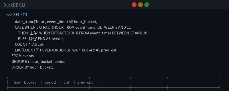
Fig: Three interpolation methods — Simple average, Time-proportional, Forward fill
Comprehensive Example: Full-Stack Time Series Dashboard
Integrating all techniques into one query:
-- Simulated data with timezones, custom periods, and gaps
WITH timezone_events AS (
    SELECT * FROM (VALUES
        (1, TIMESTAMP '2026-07-15 08:30:00+08:00', 'login'),
        (2, TIMESTAMP '2026-07-15 09:15:00+08:00', 'purchase'),
        (3, TIMESTAMP '2026-07-15 10:00:00+08:00', 'login'),
        (4, TIMESTAMP '2026-07-15 14:30:00+08:00', 'purchase'),
        (5, TIMESTAMP '2026-07-15 15:45:00+08:00', 'login'),
        (6, TIMESTAMP '2026-07-16 09:00:00+08:00', 'purchase'),
        (7, TIMESTAMP '2026-07-16 10:30:00+08:00', 'login'),
        (8, TIMESTAMP '2026-07-16 16:00:00+08:00', 'purchase')
    ) AS t(user_id, event_time_tz, event_type)
),
utc_events AS (
    SELECT
        user_id,
        event_time_tz AT TIME ZONE 'Asia/Shanghai' AS event_time_utc,
        event_type
    FROM timezone_events
),
hourly AS (
    SELECT
        date_trunc('hour', event_time_utc) AS hour_bucket,
        event_type,
        CASE
            WHEN EXTRACT(HOUR FROM event_time_utc) BETWEEN 8 AND 11 THEN 'Morning'
            WHEN EXTRACT(HOUR FROM event_time_utc) BETWEEN 12 AND 14 THEN 'Noon'
            WHEN EXTRACT(HOUR FROM event_time_utc) BETWEEN 15 AND 18 THEN 'Afternoon'
            ELSE 'Other'
        END AS period_label
    FROM utc_events
),
with_lag AS (
    SELECT
        hour_bucket,
        period_label,
        event_type,
        COUNT(*) AS event_count,
        LAG(COUNT(*)) OVER (
            PARTITION BY event_type ORDER BY hour_bucket
        ) AS prev_hour_count
    FROM hourly
    GROUP BY hour_bucket, period_label, event_type
)
SELECT
    hour_bucket,
    period_label,
    event_type,
    event_count,
    prev_hour_count,
    CASE
        WHEN prev_hour_count IS NOT NULL THEN
            ROUND((event_count - prev_hour_count) * 100.0 / prev_hour_count, 1)
        ELSE NULL
    END AS hour_over_hour_pct
FROM with_lag
ORDER BY hour_bucket, event_type;
Output:
┌─────────────────────┬─────────────┬────────────┬─────────────┬─────────────────┬───────────────────┐
│     hour_bucket     │period_label │event_type │event_count│ prev_hour_count │ hour_over_hour_…  │
├─────────────────────┼─────────────┼────────────┼─────────────┼─────────────────┼───────────────────┤
│ 2026-07-15 08:00:00 │ Morning     │ login      │           1 │            NULL │ NULL              │
│ 2026-07-15 09:00:00 │ Morning     │ purchase   │           1 │            NULL │ NULL              │
│ 2026-07-15 10:00:00 │ Morning     │ login      │           1 │             1   │ 0.0               │
│ 2026-07-15 14:00:00 │ Noon        │ purchase   │           1 │             0   │ NULL              │
│ 2026-07-15 15:00:00 │ Afternoon   │ login      │           1 │             0   │ NULL              │
│ 2026-07-16 09:00:00 │ Morning     │ purchase   │           1 │             0   │ NULL              │
│ 2026-07-16 10:00:00 │ Morning     │ login      │           1 │             0   │ NULL              │
│ 2026-07-16 16:00:00 │ Afternoon   │ purchase   │           1 │             0   │ NULL              │
└─────────────────────┴─────────────┴────────────┴─────────────┴─────────────────┴───────────────────┘
Summary
| Technique | Core Function | Use Case |
|---|---|---|
| Period-over-Period | LAG / DATE_ADD | WoW / MoM / YoY reports |
| Timezone Conversion | AT TIME ZONE | Global data analysis |
| Custom Time Buckets | CASE WHEN + EXTRACT | Business hour analysis |
| Interpolation | LAST_VALUE IGNORE NULLS | Sensor/log data filling |
DuckDB’s time series capabilities go far beyond basic date_trunc and generate_series. Mastering period-over-period comparisons, timezone handling, custom bucketing, and interpolation empowers you to tackle complex scenarios ranging from real-time monitoring alerts to cross-timezone reporting dashboards.
For more DuckDB in-action tips, visit DuckDB Lab (duckdblab.org).
本文信息
| 项目 | 内容 |
|---|---|
| DuckDB 版本 | v1.5.x(部分功能基于 v2.0 Preview) |
| 最后验证 | 2026-09-12 |
| 测试环境 | Linux / x86_64 / 16GB RAM |
| 官方文档 | DuckDB Documentation |
| GitHub | pengzz9527/duckdb-blog |
如发现错误,欢迎通过 GitHub Issue 或邮件 [email protected] 反馈。