
Why Time Series Analysis Matters
Time series data is everywhere in data analytics — daily e-commerce sales, server CPU metrics, hourly website traffic. Nearly every business scenario involves a time dimension.
Traditional databases face two major pain points when handling time series:
- Inconsistent timestamp granularity — Raw data has millisecond precision, requiring bucketing into minutes/hours/days
- Gaps in time series — Some time periods have no data, breaking continuity in visualizations
DuckDB offers three powerful tools to solve these problems elegantly: date_trunc, generate_series, and window-based rolling aggregation functions.
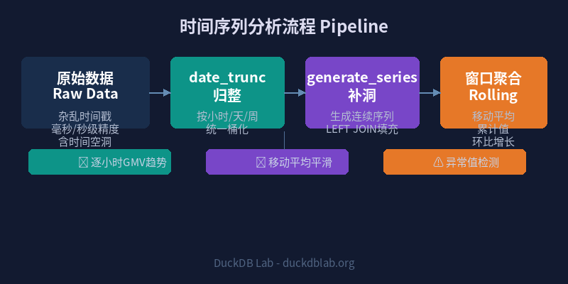
Fig: DuckDB Time Series Analysis 3-Stage Pipeline — Bucket → Fill → Roll
1. date_trunc: Timestamp Bucketing
date_trunc truncates a timestamp to a specified precision. It’s the starting point of any time series analysis — normalizing messy timestamps into uniform buckets.
Basic Syntax
date_trunc('unit', timestamp_column)
Supported unit values: 'second', 'minute', 'hour', 'day', 'week', 'month', 'quarter', 'year'.
Example: Truncate Millisecond Timestamps to Hours
SELECT
    date_trunc('hour', TIMESTAMP '2026-06-03 14:32:18.123') AS hour_bucket,
    date_trunc('day', TIMESTAMP '2026-06-03 14:32:18.123') AS day_bucket,
    date_trunc('week', TIMESTAMP '2026-06-03 14:32:18.123') AS week_bucket,
    date_trunc('month', TIMESTAMP '2026-06-03 14:32:18.123') AS month_bucket;
Result:
┌─────────────────────┬─────────────────────┬─────────────────────┬─────────────────────┐
│     hour_bucket     │     day_bucket      │     week_bucket     │    month_bucket     │
├─────────────────────┼─────────────────────┼─────────────────────┼─────────────────────┤
│ 2026-06-03 14:00:00 │ 2026-06-03 00:00:00 │ 2026-06-01 00:00:00 │ 2026-06-01 00:00:00 │
└─────────────────────┴─────────────────────┴─────────────────────┴─────────────────────┘
Note that the week_bucket starts on Monday (2026-06-01), as DuckDB defaults to ISO week (Monday start).
2. Real-World Scenario: E-Commerce Order Time Series
Let’s analyze hourly order counts and GMV (Gross Merchandise Volume) for an e-commerce platform.
Create Sample Data
CREATE TABLE orders AS
SELECT * FROM (VALUES
    (TIMESTAMP '2026-06-01 08:15:00', 1, 299.00),
    (TIMESTAMP '2026-06-01 08:42:00', 2, 159.00),
    (TIMESTAMP '2026-06-01 09:05:00', 3, 899.00),
    (TIMESTAMP '2026-06-01 09:30:00', 4, 49.90),
    (TIMESTAMP '2026-06-01 09:55:00', 5, 1299.00),
    (TIMESTAMP '2026-06-01 10:10:00', 6, 79.00),
    (TIMESTAMP '2026-06-01 10:45:00', 7, 520.00),
    (TIMESTAMP '2026-06-01 11:20:00', 8, 89.90),
    (TIMESTAMP '2026-06-01 13:00:00', 9, 249.00),
    (TIMESTAMP '2026-06-01 13:35:00', 10, 168.00),
    (TIMESTAMP '2026-06-01 14:10:00', 11, 399.00),
    (TIMESTAMP '2026-06-01 14:50:00', 12, 79.90),
    (TIMESTAMP '2026-06-01 15:25:00', 13, 1899.00),
    (TIMESTAMP '2026-06-01 16:00:00', 14, 45.00),
    (TIMESTAMP '2026-06-01 16:40:00', 15, 599.00),
    (TIMESTAMP '2026-06-02 08:30:00', 16, 129.00),
    (TIMESTAMP '2026-06-02 09:00:00', 17, 799.00),
    (TIMESTAMP '2026-06-02 09:20:00', 18, 39.00),
    (TIMESTAMP '2026-06-02 10:15:00', 19, 2399.00),
    (TIMESTAMP '2026-06-02 11:50:00', 20, 89.00)
) AS t(order_time, order_id, amount);
Hourly Aggregation
SELECT
    date_trunc('hour', order_time) AS hour_bucket,
    COUNT(*) AS order_count,
    ROUND(SUM(amount), 2) AS total_gmv,
    ROUND(AVG(amount), 2) AS avg_order_value
FROM orders
GROUP BY hour_bucket
ORDER BY hour_bucket;
Result:
┌─────────────────────┬─────────────┬───────────┬─────────────────┐
│     hour_bucket     │ order_count │ total_gmv │ avg_order_value │
├─────────────────────┼─────────────┼───────────┼─────────────────┤
│ 2026-06-01 08:00:00 │     2       │   458.00  │     229.00      │
│ 2026-06-01 09:00:00 │     3       │  2247.90  │     749.30      │
│ 2026-06-01 10:00:00 │     2       │   599.00  │     299.50      │
│ 2026-06-01 11:00:00 │     1       │    89.90  │      89.90      │
│ 2026-06-01 13:00:00 │     2       │   417.00  │     208.50      │
│ 2026-06-01 14:00:00 │     2       │   478.90  │     239.45      │
│ 2026-06-01 15:00:00 │     1       │  1899.00  │    1899.00      │
│ 2026-06-01 16:00:00 │     2       │   644.00  │     322.00      │
│ 2026-06-02 08:00:00 │     1       │   129.00  │     129.00      │
│ 2026-06-02 09:00:00 │     2       │   838.00  │     419.00      │
│ 2026-06-02 10:00:00 │     1       │  2399.00  │    2399.00      │
│ 2026-06-02 11:00:00 │     1       │    89.00  │      89.00      │
└─────────────────────┴─────────────┴───────────┴─────────────────┘
Notice the problem? June 1st has no data at 12:00 and 17:00-23:00 — the time series has gaps. If you were to chart this directly, the graph would break.
3. generate_series: Filling Time Gaps
generate_series creates a continuous time sequence, which can be used with a LEFT JOIN to fill gaps.
Generate a Continuous Hourly Series
SELECT
    generate_series AS hour_bucket
FROM generate_series(
    TIMESTAMP '2026-06-01 08:00:00',
    TIMESTAMP '2026-06-02 12:00:00',
    INTERVAL '1 hour'
);
LEFT JOIN to Fill Gaps
WITH hours AS (
    SELECT generate_series AS hour_bucket
    FROM generate_series(
        TIMESTAMP '2026-06-01 08:00:00',
        TIMESTAMP '2026-06-02 12:00:00',
        INTERVAL '1 hour'
    )
),
hourly_stats AS (
    SELECT
        date_trunc('hour', order_time) AS hour_bucket,
        COUNT(*) AS order_count,
        ROUND(SUM(amount), 2) AS total_gmv
    FROM orders
    GROUP BY hour_bucket
)
SELECT
    h.hour_bucket,
    COALESCE(s.order_count, 0) AS order_count,
    COALESCE(s.total_gmv, 0.00) AS total_gmv
FROM hours h
LEFT JOIN hourly_stats s ON h.hour_bucket = s.hour_bucket
ORDER BY h.hour_bucket;
Result:
┌─────────────────────┬─────────────┬───────────┐
│     hour_bucket     │ order_count │ total_gmv │
├─────────────────────┼─────────────┼───────────┤
│ 2026-06-01 08:00:00 │     2       │   458.00  │
│ 2026-06-01 09:00:00 │     3       │  2247.90  │
│ 2026-06-01 10:00:00 │     2       │   599.00  │
│ 2026-06-01 11:00:00 │     1       │    89.90  │
│ 2026-06-01 12:00:00 │     0       │     0.00  │  ← gap filled
│ 2026-06-01 13:00:00 │     2       │   417.00  │
│ 2026-06-01 14:00:00 │     2       │   478.90  │
│ 2026-06-01 15:00:00 │     1       │  1899.00  │
│ 2026-06-01 16:00:00 │     2       │   644.00  │
│ 2026-06-01 17:00:00 │     0       │     0.00  │  ← gap filled
│ 2026-06-01 18:00:00 │     0       │     0.00  │
│ ...                 │   ...       │    ...    │
│ 2026-06-02 08:00:00 │     1       │   129.00  │
│ 2026-06-02 09:00:00 │     2       │   838.00  │
│ 2026-06-02 10:00:00 │     1       │  2399.00  │
│ 2026-06-02 11:00:00 │     1       │    89.00  │
│ 2026-06-02 12:00:00 │     0       │     0.00  │
└─────────────────────┴─────────────┴───────────┘
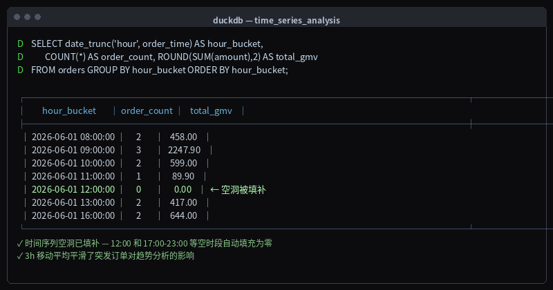
Fig: Hourly order aggregation — gaps at 12:00 and 17:00-23:00 filled with zeros by generate_series
The time series is now fully continuous, ready for charting.
4. Rolling Aggregations: Moving Averages & Cumulative Statistics
Rolling aggregation is the core technique for time series analysis, smoothing short-term fluctuations and revealing long-term trends.
4.1 3-Hour Moving Average
Use the ROWS BETWEEN window clause for sliding window calculations:
WITH hourly_gmv AS (
    SELECT
        date_trunc('hour', order_time) AS hour_bucket,
        ROUND(SUM(amount), 2) AS gmv
    FROM orders
    GROUP BY hour_bucket
)
SELECT
    hour_bucket,
    gmv,
    ROUND(AVG(gmv) OVER (
        ORDER BY hour_bucket
        ROWS BETWEEN 2 PRECEDING AND CURRENT ROW
    ), 2) AS moving_avg_3h
FROM hourly_gmv
ORDER BY hour_bucket;
Result:
┌─────────────────────┬────────┬───────────────┐
│     hour_bucket     │  gmv   │ moving_avg_3h │
├─────────────────────┼────────┼───────────────┤
│ 2026-06-01 08:00:00 │ 458.00 │    458.00     │
│ 2026-06-01 09:00:00 │2247.90 │   1352.95     │
│ 2026-06-01 10:00:00 │ 599.00 │   1101.63     │
│ 2026-06-01 11:00:00 │  89.90 │    978.93     │
│ 2026-06-01 13:00:00 │ 417.00 │    368.63     │
│ 2026-06-01 14:00:00 │ 478.90 │    328.60     │
│ 2026-06-01 15:00:00 │1899.00 │    931.63     │
│ 2026-06-01 16:00:00 │ 644.00 │   1007.30     │
│ 2026-06-02 08:00:00 │ 129.00 │    890.67     │
│ 2026-06-02 09:00:00 │ 838.00 │    537.00     │
│ 2026-06-02 10:00:00 │2399.00 │   1122.00     │
│ 2026-06-02 11:00:00 │  89.00 │   1108.67     │
└─────────────────────┴────────┴───────────────┘
The moving average smooths out the data; the large single order of 1899 at 15:00 gets distributed across the surrounding windows.
4.2 Cumulative Values (YTD / MTD)
WITH daily_gmv AS (
    SELECT
        date_trunc('day', order_time) AS day_bucket,
        ROUND(SUM(amount), 2) AS daily_gmv
    FROM orders
    GROUP BY day_bucket
)
SELECT
    day_bucket,
    daily_gmv,
    ROUND(SUM(daily_gmv) OVER (
        ORDER BY day_bucket
        ROWS BETWEEN UNBOUNDED PRECEDING AND CURRENT ROW
    ), 2) AS cumulative_gmv
FROM daily_gmv
ORDER BY day_bucket;
Result:
┌─────────────────────┬───────────┬─────────────────┐
│     day_bucket      │ daily_gmv │ cumulative_gmv  │
├─────────────────────┼───────────┼─────────────────┤
│ 2026-06-01 00:00:00 │  7089.70  │    7089.70      │
│ 2026-06-02 00:00:00 │  3455.00  │   10544.70      │
└─────────────────────┴───────────┴─────────────────┘
4.3 Month-over-Month Change Rate
WITH hourly_gmv AS (
    SELECT
        date_trunc('hour', order_time) AS hour_bucket,
        ROUND(SUM(amount), 2) AS gmv
    FROM orders
    GROUP BY hour_bucket
)
SELECT
    hour_bucket,
    gmv,
    ROUND(LAG(gmv) OVER (ORDER BY hour_bucket), 2) AS prev_hour_gmv,
    ROUND((gmv - LAG(gmv) OVER (ORDER BY hour_bucket)) /
          NULLIF(LAG(gmv) OVER (ORDER BY hour_bucket), 0) * 100, 2) AS mom_change_pct
FROM hourly_gmv
ORDER BY hour_bucket;
Result:
┌─────────────────────┬────────┬──────────────┬─────────────────┐
│     hour_bucket     │  gmv   │ prev_hour_gmv│ mom_change_pct  │
├─────────────────────┼────────┼──────────────┼─────────────────┤
│ 2026-06-01 08:00:00 │ 458.00 │     NULL     │      NULL       │
│ 2026-06-01 09:00:00 │2247.90 │    458.00    │     390.81      │
│ 2026-06-01 10:00:00 │ 599.00 │   2247.90    │     -73.35      │
│ 2026-06-01 11:00:00 │  89.90 │    599.00    │     -84.99      │
│ 2026-06-01 13:00:00 │ 417.00 │     89.90    │     363.85      │
│ 2026-06-01 14:00:00 │ 478.90 │    417.00    │      14.84      │
│ 2026-06-01 15:00:00 │1899.00 │    478.90    │     296.53      │
│ 2026-06-01 16:00:00 │ 644.00 │   1899.00    │     -66.09      │
└─────────────────────┴────────┴──────────────┴─────────────────┘
5. Advanced Example: Server Monitoring Metrics
Let’s analyze a server monitoring scenario — CPU usage over the past 7 days.
Create Simulated Monitoring Data
CREATE TABLE cpu_metrics AS
SELECT
    '2026-06-03 08:00:00'::TIMESTAMP + INTERVAL (i || ' minutes') AS ts,
    30 + random() * 40 AS cpu_usage,
    1024 + random() * 2048 AS memory_mb
FROM generate_series(0, 1439) AS t(i);  -- 24 hours of minute-level data
15-Minute Rolling Window Analysis
SELECT
    date_trunc('hour', ts) AS hour_bucket,
    ROUND(AVG(cpu_usage), 1) AS avg_cpu,
    ROUND(MAX(cpu_usage), 1) AS max_cpu,
    ROUND(MIN(cpu_usage), 1) AS min_cpu,
    ROUND(AVG(memory_mb), 0) AS avg_memory_mb
FROM cpu_metrics
GROUP BY hour_bucket
ORDER BY hour_bucket;
Sliding Window Anomaly Detection
Use LAG and LEAD for CPU spike detection:
WITH cpu_by_minute AS (
    SELECT
        ts,
        ROUND(cpu_usage, 1) AS cpu_usage,
        ROUND(AVG(cpu_usage) OVER (
            ORDER BY ts
            ROWS BETWEEN 5 PRECEDING AND 1 PRECEDING
        ), 1) AS baseline
    FROM cpu_metrics
)
SELECT
    ts,
    cpu_usage,
    baseline,
    ROUND(cpu_usage - baseline, 1) AS deviation
FROM cpu_by_minute
WHERE cpu_usage > baseline * 1.5  -- 50% above baseline = anomaly
ORDER BY deviation DESC
LIMIT 10;
6. Performance Optimization Tips
When processing large-scale time series data, these techniques can significantly improve query performance:
| Technique | Description | Best For |
|---|---|---|
| Table Partitioning | Partition by time range (daily/monthly) | Millions+ rows |
| Materialized Aggregations | Use CREATE TABLE AS to pre-aggregate hourly stats | Fixed-granularity repeated queries |
| Ordering | ORDER BY ts on timestamp column | Frequent range scans |
| Parquet Partitioning | Store by year/month/day | Hot/cold data separation |
Use ORDER BY to Accelerate Timestamp Scans
-- Adding ORDER BY during table creation speeds up range queries
CREATE TABLE orders_partitioned AS
SELECT * FROM read_parquet('orders.parquet')
ORDER BY order_time;
Summary
DuckDB’s time series analysis capabilities can be summarized in three layers:
- Bucketing (date_trunc) — Normalize fine-grained timestamps into uniform buckets, the starting point of any time series analysis
- Gap Filling (generate_series) — Generate continuous time sequences and LEFT JOIN to fill data gaps, ensuring complete charts
- Rolling Analysis (Window Functions) — Moving averages, cumulative values, and MoM changes to reveal underlying trends
Combined, these three tools handle over 90% of time series analysis needs. Whether it’s e-commerce GMV monitoring, server alerting, or IoT sensor data processing, this methodology applies.
💡 Try it yourself! Replace the
orderstable above with your own business data (logs, transactions, sensor readings) and run the full time series analysis pipeline immediately.
For more DuckDB in Action tips, follow Olap Studio (duckdblab.org)