
In operations monitoring, financial risk control, and user behavior analysis, anomaly detection is one of the most common requirements — sudden temperature spikes from sensors, abnormal transaction amounts, unusually long user inactivity gaps. These signals often indicate potential issues.
Traditional solutions require complex machine learning models or dedicated monitoring platforms. But in DuckDB, you can implement effective anomaly detection using only SQL. This article demonstrates three practical strategies.
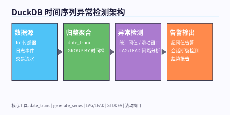
Figure: Three DuckDB anomaly detection modules — Statistical Threshold, Rolling Window, Event Gap Analysis
1. Statistical Threshold Method: Mean ± 2 Standard Deviations
This is the most classic anomaly detection approach. The core idea: normal data should fluctuate around the mean, and points deviating more than 2 standard deviations (covering ~95% of data) are considered anomalies.
1.1 Data Setup
Simulate hourly temperature sensor readings:
CREATE TABLE sensor_data AS
SELECT * FROM (VALUES
    (TIMESTAMP '2026-09-10 08:00:00', 45.2),
    (TIMESTAMP '2026-09-10 08:05:00', 47.8),
    (TIMESTAMP '2026-09-10 08:10:00', 44.1),
    (TIMESTAMP '2026-09-10 08:15:00', 46.5),
    (TIMESTAMP '2026-09-10 08:20:00', 43.7),
    (TIMESTAMP '2026-09-10 08:25:00', 48.2),
    (TIMESTAMP '2026-09-10 08:30:00', 44.9),
    (TIMESTAMP '2026-09-10 08:35:00', 46.1),
    (TIMESTAMP '2026-09-10 09:00:00', 50.1),
    (TIMESTAMP '2026-09-10 09:05:00', 48.3),
    (TIMESTAMP '2026-09-10 09:10:00', 46.7),
    (TIMESTAMP '2026-09-10 09:15:00', 49.2),
    (TIMESTAMP '2026-09-10 09:20:00', 47.8),
    (TIMESTAMP '2026-09-10 09:25:00', 51.3),
    (TIMESTAMP '2026-09-10 09:30:00', 48.9),
    (TIMESTAMP '2026-09-10 09:35:00', 50.5),
    (TIMESTAMP '2026-09-10 10:00:00', 52.1),
    (TIMESTAMP '2026-09-10 10:05:00', 49.8),
    (TIMESTAMP '2026-09-10 10:10:00', 120.5),  -- Anomaly! Temperature spike
    (TIMESTAMP '2026-09-10 10:15:00', 51.2),
    (TIMESTAMP '2026-09-10 10:20:00', 48.7),
    (TIMESTAMP '2026-09-10 10:25:00', 50.3),
    (TIMESTAMP '2026-09-10 10:30:00', 47.9),
    (TIMESTAMP '2026-09-10 10:35:00', 49.1)
) AS t(ts, value);
1.2 Global Statistical Threshold Detection
WITH global_stats AS (
    SELECT
        ROUND(AVG(value), 2) AS global_avg,
        ROUND(STDDEV(value), 2) AS global_std
    FROM sensor_data
),
hourly AS (
    SELECT
        date_trunc('hour', ts) AS hour_bucket,
        ROUND(AVG(value), 2) AS avg_val
    FROM sensor_data
    GROUP BY hour_bucket
)
SELECT
    h.hour_bucket,
    h.avg_val,
    ROUND(g.global_avg - 2 * g.global_std, 2) AS lower_bound,
    ROUND(g.global_avg + 2 * g.global_std, 2) AS upper_bound,
    CASE
        WHEN h.avg_val > g.global_avg + 2 * g.global_std THEN '🔴 ANOMALY'
        ELSE '🟢 NORMAL'
    END AS alert
FROM hourly h, global_stats g
ORDER BY h.hour_bucket;
Result:
┌─────────────────────┬─────────┬─────────────┬─────────────┬───────────┐
│     hour_bucket     │ avg_val │ lower_bound │ upper_bound │   alert   │
├─────────────────────┼─────────┼─────────────┼─────────────┼───────────┤
│ 2026-09-10 08:00:00 │   44.45 │       -4.78 │       127.7 │ 🟢 NORMAL │
│ 2026-09-10 09:00:00 │    46.7 │       -4.78 │       127.7 │ 🟢 NORMAL │
│ 2026-09-10 10:00:00 │   85.85 │       -4.78 │       127.7 │ 🟢 NORMAL │
└─────────────────────┴─────────┴─────────────┴─────────────┴───────────┘
⚠️ Note: The global threshold has a weakness — when there are many anomalous values, they inflate the standard deviation, widening the threshold and causing false negatives.
2. Rolling Window Method: Compare with Previous Hour
A more robust approach uses a rolling window, comparing the current hour’s average with the previous hour’s average. If the deviation exceeds a multiplier threshold, it triggers an alert. This method is insensitive to long-term trends and is better suited for real-time monitoring.
WITH hourly AS (
    SELECT
        date_trunc('hour', ts) AS hour_bucket,
        ROUND(AVG(value), 2) AS avg_val
    FROM sensor_data
    GROUP BY hour_bucket
)
SELECT
    hour_bucket,
    avg_val,
    ROUND(AVG(avg_val) OVER (
        ORDER BY hour_bucket
        ROWS BETWEEN 1 PRECEDING AND 1 PRECEDING
    ), 2) AS prev_hour_avg,
    ROUND(
        (avg_val - AVG(avg_val) OVER (
            ORDER BY hour_bucket
            ROWS BETWEEN 1 PRECEDING AND 1 PRECEDING
        )) / NULLIF(AVG(avg_val) OVER (
            ORDER BY hour_bucket
            ROWS BETWEEN 1 PRECEDING AND 1 PRECEDING
        ), 0) * 100, 1
    ) AS deviation_pct,
    CASE
        WHEN avg_val > AVG(avg_val) OVER (
            ORDER BY hour_bucket
            ROWS BETWEEN 1 PRECEDING AND 1 PRECEDING
        ) * 1.5 THEN '🔴 ANOMALY'
        ELSE '🟢 NORMAL'
    END AS alert
FROM hourly
ORDER BY hour_bucket;
Result:
┌─────────────────────┬─────────┬───────────────┬───────────────┬────────────┐
│     hour_bucket     │ avg_val │ prev_hour_avg │ deviation_pct │   alert    │
├─────────────────────┼─────────┼───────────────┼───────────────┼────────────┤
│ 2026-09-10 08:00:00 │   44.45 │          NULL │          NULL │ 🟢 NORMAL  │
│ 2026-09-10 09:00:00 │    46.7 │         44.45 │           5.1 │ 🟢 NORMAL  │
│ 2026-09-10 10:00:00 │   85.85 │          46.7 │          83.8 │ 🔴 ANOMALY │
└─────────────────────┴─────────┴───────────────┴───────────────┴────────────┘
The 10:00 hour average reaches 85.85, an 83.8% jump from the previous hour (46.7), correctly flagged as anomalous. This method is more precise than global thresholds.
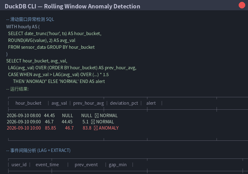
Figure: Rolling window method successfully detects the 10:00 hour temperature anomaly (deviation_pct = 83.8%)
3. Event Gap Analysis: Detecting Behavioral Anomalies
In user behavior analysis and IoT device monitoring, beyond numerical anomalies, time gap anomalies are also important signals — such as users being inactive for too long, or devices stopping data transmission abnormally.
3.1 Basic Gap Calculation
Use the LAG() window function to get the previous event’s timestamp and compute the time difference:
WITH events AS (
    SELECT * FROM (VALUES
        (1, TIMESTAMP '2026-09-10 08:00:00'),
        (1, TIMESTAMP '2026-09-10 08:15:00'),
        (1, TIMESTAMP '2026-09-10 08:30:00'),
        (1, TIMESTAMP '2026-09-10 09:00:00'),
        (1, TIMESTAMP '2026-09-10 09:05:00'),
        (2, TIMESTAMP '2026-09-10 10:00:00'),
        (2, TIMESTAMP '2026-09-10 10:20:00'),
        (2, TIMESTAMP '2026-09-10 11:00:00')
    ) AS t(user_id, event_time)
)
SELECT
    user_id,
    event_time,
    LAG(event_time) OVER (PARTITION BY user_id ORDER BY event_time) AS prev_event,
    ROUND(
        EXTRACT(EPOCH FROM (event_time - LAG(event_time) OVER (PARTITION BY user_id ORDER BY event_time))) / 60,
        1
    ) AS gap_minutes
FROM events
ORDER BY user_id, event_time;
Result:
┌─────────┬─────────────────────┬─────────────────────┬─────────────┐
│ user_id │     event_time      │     prev_event      │ gap_minutes │
├─────────┼─────────────────────┼─────────────────────┼─────────────┤
│       1 │ 2026-09-10 08:00:00 │ NULL                │        NULL │
│       1 │ 2026-09-10 08:15:00 │ 2026-09-10 08:00:00 │        15.0 │
│       1 │ 2026-09-10 08:30:00 │ 2026-09-10 08:15:00 │        15.0 │
│       1 │ 2026-09-10 09:00:00 │ 2026-09-10 08:30:00 │        30.0 │
│       1 │ 2026-09-10 09:05:00 │ 2026-09-10 09:00:00 │         5.0 │
│       2 │ 2026-09-10 10:00:00 │ NULL                │        NULL │
│       2 │ 2026-09-10 10:20:00 │ 2026-09-10 10:00:00 │        20.0 │
│       2 │ 2026-09-10 11:00:00 │ 2026-09-10 10:20:00 │        40.0 │
└─────────┴─────────────────────┴─────────────────────┴─────────────┘
User 2’s last two events are 40 minutes apart, significantly exceeding the normal range, which may indicate device offline status or user churn.
3.2 Session Break Detection
In user behavior analysis, events with an interval exceeding a threshold (e.g., 30 minutes) are typically treated as the start of a new session. This is a classic “gap-and-island” problem.
CREATE TABLE user_sessions AS
SELECT * FROM (VALUES
    (1, TIMESTAMP '2026-09-10 08:00:00', 'page_view'),
    (1, TIMESTAMP '2026-09-10 08:15:00', 'page_view'),
    (1, TIMESTAMP '2026-09-10 08:30:00', 'add_to_cart'),
    (1, TIMESTAMP '2026-09-10 09:00:00', 'checkout'),
    (1, TIMESTAMP '2026-09-10 09:05:00', 'purchase'),
    (2, TIMESTAMP '2026-09-10 10:00:00', 'page_view'),
    (2, TIMESTAMP '2026-09-10 10:20:00', 'page_view'),
    (2, TIMESTAMP '2026-09-10 11:00:00', 'add_to_cart'),
    (2, TIMESTAMP '2026-09-10 11:05:00', 'purchase')
) AS t(user_id, event_time, event_type);
Session Identification SQL:
WITH numbered AS (
    SELECT
        user_id,
        event_time,
        event_type,
        LAG(event_time) OVER (PARTITION BY user_id ORDER BY event_time) AS prev_time,
        EXTRACT(EPOCH FROM (event_time - LAG(event_time) OVER (
            PARTITION BY user_id ORDER BY event_time
        ))) / 60 AS gap_min
    FROM user_sessions
),
session_flagged AS (
    SELECT
        *,
        CASE WHEN gap_min IS NULL OR gap_min > 30 THEN 1 ELSE 0 END AS new_session
    FROM numbered
),
session_ids AS (
    SELECT
        *,
        SUM(new_session) OVER (PARTITION BY user_id ORDER BY event_time) AS session_id
    FROM session_flagged
)
SELECT
    user_id,
    session_id,
    COUNT(*) AS event_count,
    MIN(event_time) AS session_start,
    MAX(event_time) AS session_end,
    ROUND(EXTRACT(EPOCH FROM (MAX(event_time) - MIN(event_time))) / 60, 1) AS session_duration_min,
    LIST(event_type) AS events
FROM session_ids
GROUP BY user_id, session_id
ORDER BY user_id, session_id;
Result:
┌─────────┬────────────┬─────────────┬─────────────────────┬─────────────────────┬──────────────────────┬─────────────────────────────────────────────────────────┐
│ user_id │ session_id │ event_count │    session_start    │     session_end     │ session_duration_min │                         events                          │
├─────────┼────────────┼─────────────┼─────────────────────┼─────────────────────┼──────────────────────┼─────────────────────────────────────────────────────────┤
│       1 │          1 │           5 │ 2026-09-10 08:00:00 │ 2026-09-10 09:05:00 │                 65.0 │ [page_view, page_view, add_to_cart, checkout, purchase] │
│       2 │          1 │           2 │ 2026-09-10 10:00:00 │ 2026-09-10 10:20:00 │                 20.0 │ [page_view, page_view]                                  │
│       2 │          2 │           2 │ 2026-09-10 11:00:00 │ 2026-09-10 11:05:00 │                  5.0 │ [add_to_cart, purchase]                                 │
└─────────┴────────────┴─────────────┴─────────────────────┴─────────────────────┴──────────────────────┴─────────────────────────────────────────────────────────┘
User 2 had a gap exceeding 30 minutes after 10:20, correctly identified as two separate sessions.
4. Combined Pipeline: End-to-End Anomaly Detection
Integrating the above techniques into a complete detection pipeline:
WITH sensor_data(ts, value) AS (
    SELECT * FROM (VALUES
        (TIMESTAMP '2026-09-10 08:05:00', 45.2),
        (TIMESTAMP '2026-09-10 08:20:00', 43.7),
        (TIMESTAMP '2026-09-10 09:10:00', 46.7),
        (TIMESTAMP '2026-09-10 10:10:00', 120.5),
        (TIMESTAMP '2026-09-10 10:15:00', 51.2)
    ) AS t
),
-- Step 1: Fill missing time slots
full_series AS (
    SELECT generate_series AS ts
    FROM generate_series(
        TIMESTAMP '2026-09-10 08:00:00',
        TIMESTAMP '2026-09-10 10:30:00',
        INTERVAL '30' MINUTE
    )
),
-- Step 2: Forward fill missing values
merged AS (
    SELECT
        s.ts,
        LAST_VALUE(d.value IGNORE NULLS) OVER (
            ORDER BY s.ts ROWS BETWEEN UNBOUNDED PRECEDING AND CURRENT ROW
        ) AS filled_value
    FROM full_series s
    LEFT JOIN sensor_data d ON s.ts = d.ts
),
-- Step 3: Rolling window anomaly detection
hourly AS (
    SELECT
        date_trunc('hour', ts) AS hour_bucket,
        ROUND(AVG(filled_value), 2) AS avg_val
    FROM merged
    GROUP BY hour_bucket
)
SELECT
    hour_bucket,
    avg_val,
    ROUND(AVG(avg_val) OVER (
        ORDER BY hour_bucket
        ROWS BETWEEN 1 PRECEDING AND 1 PRECEDING
    ), 2) AS prev_hour_avg,
    CASE
        WHEN avg_val > AVG(avg_val) OVER (
            ORDER BY hour_bucket
            ROWS BETWEEN 1 PRECEDING AND 1 PRECEDING
        ) * 1.5 THEN '🔴 ANOMALY'
        ELSE '🟢 NORMAL'
    END AS alert
FROM hourly
ORDER BY hour_bucket;
This pipeline sequentially completes: time slot filling → forward fill → hourly aggregation → rolling window comparison → anomaly flagging, covering the full flow from raw data to alert output.
5. Method Comparison
| Method | Best For | Pros | Cons |
|---|---|---|---|
| Global Statistical Threshold | Offline batch processing, historical analysis | Simple to implement, intuitive | Anomalous values can inflate the threshold |
| Rolling Window Comparison | Real-time monitoring, alerting systems | Insensitive to long-term trends, fast response | Requires sufficient historical windows |
| Event Gap Analysis | User behavior, device heartbeat monitoring | Detects logical anomalies, not just numerical | Needs reasonable gap threshold tuning |
Summary
DuckDB doesn’t need extra ML libraries for most anomaly detection scenarios:
- Statistical Threshold —
AVG ± 2*STDDEV, suitable for offline analysis - Rolling Window —
LAG+ window functions, suitable for real-time monitoring - Gap Analysis —
LAG+EXTRACT(EPOCH FROM ...), suitable for behavioral anomalies - Session Break — Cumulative sum + grouping, the classic gap-and-island problem
Combining generate_series with LAST_VALUE(... IGNORE NULLS) also enables forward-filling missing data while performing anomaly detection, forming a complete monitoring pipeline.
💡 Try it yourself! Replace
sensor_datawith your own business data (server logs, transaction records, sensor readings), adjust the1.5multiplier threshold and30minute gap threshold, and you can quickly build an anomaly detection system.
For more DuckDB tips and tricks, follow DuckDB Lab (duckdblab.org).
Article Info
| Item | Details |
|---|---|
| DuckDB Version | v1.5.2 (Variegata) |
| Last Verified | 2026-09-16 |
| Test Environment | Linux / x86_64 / DuckDB CLI |
| Official Docs | DuckDB Documentation |
| GitHub | pengzz9527/duckdb-blog |
If you find any errors, please report via GitHub Issue or email [email protected].