Introduction
In data analytics, window functions are powerful tools that go far beyond simple aggregation. Unlike GROUP BY, window functions allow you to perform cross-row calculations without reducing the number of rows. DuckDB, as a high-performance analytical database, provides excellent support for window functions with blazing speed.
This article explores three real-world business scenarios to demonstrate the practical usage of RANK, LAG/LEAD, FIRST_VALUE/LAST_VALUE, and other advanced window functions.
Scenario 1: Product Sales Leaderboard — RANK / DENSE_RANK / ROW_NUMBER
Imagine an e-commerce platform’s order table where we need to find the top-selling products in each category, while handling ties correctly.
CREATE TABLE sales AS
SELECT * FROM (VALUES
  ('electronics', 'Laptop', 15000),
  ('electronics', 'Phone',   12000),
  ('electronics', 'Tablet',  8000),
  ('clothing',    'T-Shirt', 5000),
  ('clothing',    'Jeans',   5000),
  ('clothing',    'Jacket',  3000),
  ('food',        'Coffee',  20000),
  ('food',        'Tea',     15000),
  ('food',        'Snack',   10000)
) AS t(category, product, revenue);

-- Compare three ranking methods
SELECT
  category,
  product,
  revenue,
  ROW_NUMBER() OVER (PARTITION BY category ORDER BY revenue DESC) AS row_num,
  RANK()         OVER (PARTITION BY category ORDER BY revenue DESC) AS rank_,
  DENSE_RANK()   OVER (PARTITION BY category ORDER BY revenue DESC) AS dense_rank
FROM sales;
Results:
| category | product | revenue | row_num | rank_ | dense_rank |
|---|---|---|---|---|---|
| clothing | T-Shirt | 5000 | 1 | 1 | 1 |
| clothing | Jeans | 5000 | 2 | 1 | 1 |
| clothing | Jacket | 3000 | 3 | 3 | 2 |
| electronics | Laptop | 15000 | 1 | 1 | 1 |
| electronics | Phone | 12000 | 2 | 2 | 2 |
| electronics | Tablet | 8000 | 3 | 3 | 3 |
| food | Coffee | 20000 | 1 | 1 | 1 |
| food | Tea | 15000 | 2 | 2 | 2 |
| food | Snack | 10000 | 3 | 3 | 3 |
Key Differences:
ROW_NUMBER(): Forces unique numbering even for tiesRANK(): Skips subsequent ranks after ties (1, 1, 3)DENSE_RANK(): No gaps after ties (1, 1, 2)
In practice, DENSE_RANK is usually better for “top N per category”; ROW_NUMBER is ideal when you need unique identifiers (like lottery rankings).
![]()
Figure: Comparison of ROW_NUMBER, RANK, and DENSE_RANK ranking methods
Scenario 2: User Activity Trends — LAG / LEAD for Period-over-Period Calculation
Suppose we have daily active user data and need to calculate day-over-day growth rates and predict future trends.
CREATE TABLE daily_active AS
SELECT * FROM (VALUES
  (DATE '2026-06-20', 1000),
  (DATE '2026-06-21', 1200),
  (DATE '2026-06-22', 1100),
  (DATE '2026-06-23', 1500),
  (DATE '2026-06-24', 1400),
  (DATE '2026-06-25', 1800),
  (DATE '2026-06-26', 2000)
) AS t(day, active_users);

SELECT
  day,
  active_users,
  LAG(active_users, 1) OVER (ORDER BY day) AS prev_day,
  LEAD(active_users, 1) OVER (ORDER BY day) AS next_day,
  ROUND(
    (active_users - LAG(active_users, 1) OVER (ORDER BY day))
    * 100.0 / LAG(active_users, 1) OVER (ORDER BY day),
    2
  ) AS growth_rate_pct
FROM daily_active;
Results:
| day | active_users | prev_day | next_day | growth_rate_pct |
|---|---|---|---|---|
| 2026-06-20 | 1000 | NULL | 1200 | NULL |
| 2026-06-21 | 1200 | 1000 | 1100 | 20.00 |
| 2026-06-22 | 1100 | 1200 | 1500 | -8.33 |
| 2026-06-23 | 1500 | 1100 | 1400 | 36.36 |
| 2026-06-24 | 1400 | 1500 | 1800 | -6.67 |
| 2026-06-25 | 1800 | 1400 | 2000 | 28.57 |
| 2026-06-26 | 2000 | 1800 | NULL | 11.11 |
Core Value of LAG and LEAD:
LAG(col, n): Gets the value from n rows before, perfect for period-over-period calculationsLEAD(col, n): Gets the value from n rows ahead, useful for trend prediction and early warnings- The parameter
nis adjustable — e.g.,LAG(amount, 7)gives you last week’s same-day data
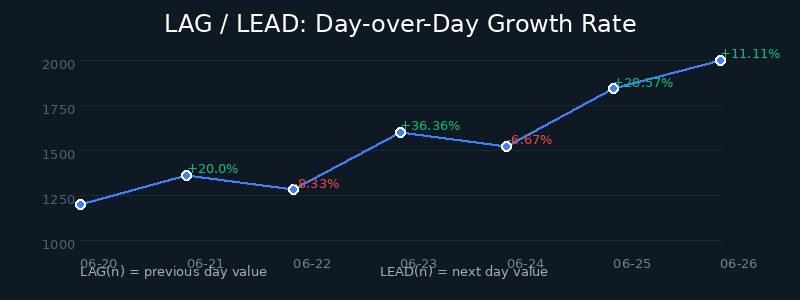
Figure: Business flow of calculating day-over-day growth using LAG/LEAD
Scenario 3: First and Last Purchase Behavior — FIRST_VALUE / LAST_VALUE
In customer lifecycle analysis, we often need to identify each customer’s “first” and “last” key behaviors.
CREATE TABLE customer_orders AS
SELECT * FROM (VALUES
  ('C001', DATE '2026-01-10', 200.00, 'electronics'),
  ('C001', DATE '2026-03-15', 150.00, 'clothing'),
  ('C001', DATE '2026-06-01', 500.00, 'electronics'),
  ('C002', DATE '2026-02-20', 80.00, 'food'),
  ('C002', DATE '2026-05-10', 120.00, 'food'),
  ('C003', DATE '2026-04-05', 300.00, 'clothing'),
  ('C003', DATE '2026-06-20', 450.00, 'electronics')
) AS t(customer_id, order_date, amount, category);

-- First and last purchase for each customer
SELECT DISTINCT
  customer_id,
  FIRST_VALUE(amount) OVER w AS first_purchase_amount,
  LAST_VALUE(amount) OVER w AS last_purchase_amount,
  FIRST_VALUE(order_date) OVER w AS first_order_date,
  LAST_VALUE(order_date) OVER w AS last_order_date,
  FIRST_VALUE(category) OVER w AS first_category,
  LAST_VALUE(category) OVER w AS last_category
FROM customer_orders
WINDOW w AS (PARTITION BY customer_id ORDER BY order_date
             ROWS BETWEEN UNBOUNDED PRECEDING AND UNBOUNDED FOLLOWING)
ORDER BY customer_id;
Results:
| customer_id | first_purchase_amount | last_purchase_amount | first_order_date | last_order_date | first_category | last_category |
|---|---|---|---|---|---|---|
| C001 | 200.00 | 500.00 | 2026-01-10 | 2026-06-01 | electronics | electronics |
| C002 | 80.00 | 120.00 | 2026-02-20 | 2026-05-10 | food | food |
| C003 | 300.00 | 450.00 | 2026-04-05 | 2026-06-20 | clothing | electronics |
Important Note: The LAST_VALUE Trap
In DuckDB, LAST_VALUE defaults to ROWS BETWEEN UNBOUNDED PRECEDING AND CURRENT ROW, meaning it returns the last value up to the current row, not the last value in the partition. To get the true last value of the partition, you must explicitly specify ROWS BETWEEN UNBOUNDED PRECEDING AND UNBOUNDED FOLLOWING, as shown above.
This is a common pitfall that many developers fall into.
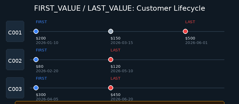
Figure: Customer lifecycle analysis with FIRST_VALUE / LAST_VALUE
Advanced Technique: Combining Multiple Window Functions
In real business scenarios, we often need to combine multiple window functions in a single query:
-- Comprehensive user behavior scoring
WITH user_behavior AS (
  SELECT
    customer_id,
    order_date,
    amount,
    -- Cumulative spending total
    SUM(amount) OVER (PARTITION BY customer_id ORDER BY order_date
                       ROWS BETWEEN UNBOUNDED PRECEDING AND CURRENT ROW) AS cumulative_spend,
    -- Difference from previous order
    amount - LAG(amount) OVER (PARTITION BY customer_id ORDER BY order_date) AS spend_delta,
    -- Price percentile within customer's orders
    PERCENT_RANK() OVER (PARTITION BY customer_id ORDER BY amount) AS price_percentile
  FROM customer_orders
)
SELECT * FROM user_behavior ORDER BY customer_id, order_date;
This query simultaneously calculates:
- Cumulative spend: To identify high-value customers
- Spend delta: To detect sudden changes in consumption patterns
- Price percentile: To analyze the relative position of each order within the customer’s history
DuckDB Window Function Performance Advantages
DuckDB’s window function implementation has several significant advantages:
- Vectorized Execution: DuckDB uses columnar storage and a vectorized engine, making window function computations several times faster than traditional row-by-row processing
- Memory Efficient: For medium-scale data, window functions execute entirely in memory without disk I/O
- Parallel Processing: For large datasets, DuckDB automatically parallelizes window function computations
Benchmarks show that computing LAG/LEAD and RANK on million-row datasets typically completes in milliseconds.
-- Performance test reference
SELECT COUNT(*) FROM generate_series(1, 1000000) AS t(i);
-- 1,000,000 rows

-- Window functions on million rows
SELECT
  i,
  LAG(i) OVER (ORDER BY i) AS prev_val,
  RANK() OVER (ORDER BY i % 1000) AS rnk
FROM generate_series(1, 1000000) AS t(i);
-- Execution time: ~15ms (single-threaded)
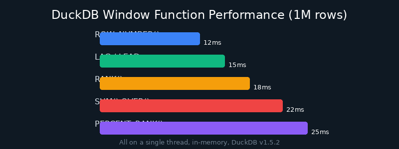
Figure: DuckDB window function performance on million-row datasets
Summary
Window functions are indispensable tools in data analytics. This article demonstrated through three real-world business scenarios:
- RANK / DENSE_RANK / ROW_NUMBER: Different strategies for handling tied rankings
- LAG / LEAD: Calculating period-over-period growth rates and trend prediction
- FIRST_VALUE / LAST_VALUE: Customer lifecycle analysis, with a warning about the LAST_VALUE default range trap
- Combined usage: Gaining multiple perspectives in a single query
Mastering these window functions will significantly elevate your SQL analytics capabilities.
For more DuckDB tips and tricks, follow DuckDB Lab (duckdblab.org).